Production Analytics Guide
Overview
What is Production Analytics?
Production Analytics is MachineMetrics' powerful benchmarking tool designed to optimize quoting and costing by comparing actual production performance against planned estimates. This tool empowers CFOs, estimators, and production planners to make data-driven decisions about pricing, capacity, and profitability.
Primary Goal: Provide real, historical data on how long jobs actually take versus how long they were planned to take, enabling you to continuously improve quote accuracy and understand true job profitability.
Who Uses This
Target Users:
- CFOs & Finance Teams: Analyze true job costs and profitability
- Estimators & Quoting Teams: Improve quote accuracy with real performance data
- Production Planners: Benchmark operations and optimize scheduling
- Operations Managers: Identify improvement opportunities based on actual vs planned performance
Key Business Questions Answered
Production Analytics helps you answer critical questions like:
-
"Are we making or losing money on this job?"
- Compare actual labor hours and costs against quoted estimates
- Calculate true per-part cost including downtime and inefficiencies
-
"How long does this operation really take?"
- See median, mode, and average cycle times from real production runs
- Compare actual performance against ERP standards
-
"Where are we losing time and money?"
- Identify top downtime reasons by duration
- Quantify the cost impact of performance losses
-
"Should we update our quotes for this part?"
- Benchmark current runs against historical performance
- Use real data to adjust future estimates
-
"How consistent is our process?"
- Analyze cycle time variability and stability
- Identify operations with high variance that impact scheduling
Why Production Analytics
The Business Problem
Most manufacturers quote jobs based on:
- ERP standards (often outdated or inaccurate)
- Estimator experience and intuition
- Historical data from paper logs (incomplete or unreliable)
- Assumption that planned time = actual time
The Reality: Actual production rarely matches the plan. Without visibility into what actually happens on the shop floor, you're quoting blind.
Common Issues:
- ❌ Quotes based on ideal conditions (no downtime, perfect cycles, experienced operators)
- ❌ No visibility into where time is lost (setup, tool changes, waiting for material, quality issues)
- ❌ Can't compare current job performance to historical runs
- ❌ Don't know true per-part cost until after the fact (too late to adjust)
- ❌ Manual data collection is time-consuming and prone to errors
The Solution
Production Analytics provides:
- ✅ Real-time benchmarking by part operation
- ✅ Actual vs planned comparisons for every metric (cycle time, OEE, downtime)
- ✅ Historical run comparison to see performance trends over time
- ✅ Cost analysis showing true profitability including losses
- ✅ Automatic data collection from machine controls (no manual logging)
Result: Make informed decisions about pricing, capacity, and process improvements backed by real production data.
Accessing Production Analytics
Navigation
From Main Menu (Primary Method):
- Expand Production in the left-hand navigation menu
- Select Analytics
- You will see options to view data by:
- Search by part operation - Find specific operations
- Completed work cycle times - Analyze finished jobs
- In progress cycle times - Monitor active jobs
- Completed work OEE - Review OEE for finished jobs
- In progress OEE - Track OEE for active jobs
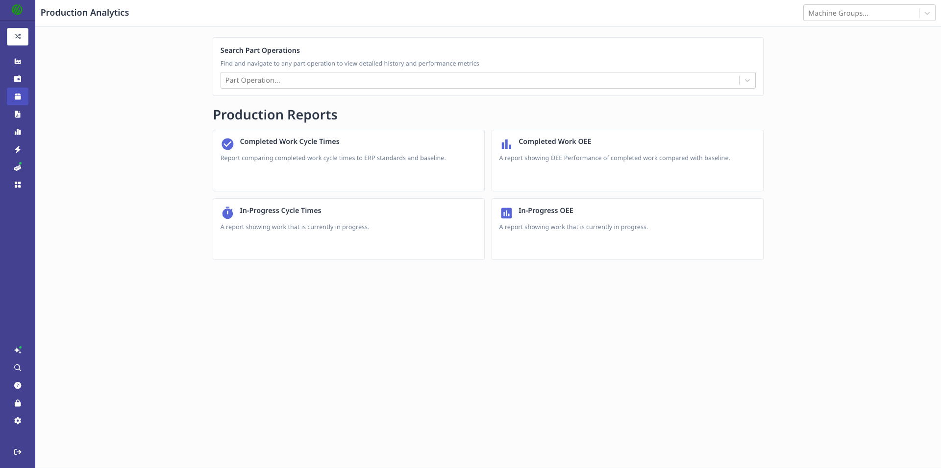
Access Production Analytics from the Production menu in the left-hand navigation. Select how you want to analyze your data - by part operation, cycle times, or OEE for completed or in-progress work.
From Machine View (Alternative Method):
- Navigate to Machines → Select a machine
- Scroll to the bottom of the Overview page
- You will see all operations that have been run on that machine in the selected time period
- Click on any operation to view its analytics
Note: Operations are created and managed from the Production → Operations page. This guide focuses solely on analyzing production data, not managing operations. See the Operations Management guide for details on creating and importing operations.
History Button - Comparing Previous Runs
Overview
The History button at the top of Production Analytics is one of the most powerful features for benchmarking and optimization. It allows you to see all previous runs of the selected operation and compare performance over time.
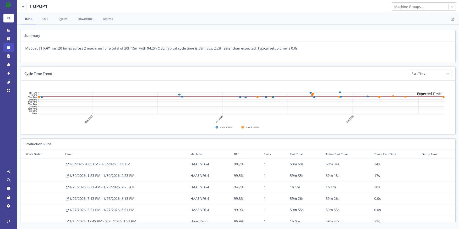
The History view displays all previous production runs for the selected operation, showing OEE, availability, performance, quality, cycle times, and downtime for each run. Use this to identify trends, compare operator performance, and track process improvements over time.
Using History to Optimize Quotes
How It Works:
- Open Production Analytics for a specific operation
- Click History button at the top of the page
- View table of all historical runs with key metrics
Data Displayed:
- Run Date: When the operation ran
- Machine: Which machine was used
- Operator: Who ran the operation
- Parts Produced: Good parts and rejected parts
- OEE %: Overall Equipment Effectiveness
- Availability %
- Performance %
- Quality %
- Cycle Times:
- Actual median cycle time
- Expected cycle time
- Variance from expected
- Downtime: Total downtime and top reasons
- Setup Time: Actual setup time vs planned
Key Use Cases
1. Benchmarking Current Run Against Historical Performance
Compare the current production run to past runs:
- Is current cycle time faster or slower than typical?
- Is OEE improving or declining over time?
- Are we experiencing more downtime than usual?
Example:
Operation: Housing Rough Turn (Part 1077280-OP10)

Historical Runs:
- Jan 15: OEE 88%, Cycle Time 17m 14s, 500 parts
- Feb 3: OEE 85%, Cycle Time 18m 02s, 500 parts
- Feb 20: OEE 90%, Cycle Time 16m 45s, 500 parts ← Best run
- Current: OEE 86%, Cycle Time 17m 30s, 500 parts in progress

Analysis: Current run is slightly below best performance.
Investigate what was different on Feb 20 run.
2. Operator Performance Comparison
Identify training opportunities or best practices:
- Which operators consistently achieve best cycle times?
- Is there significant variance between operators?
- Can top performers share techniques with others?
Example:
Operation: Mill Flats (Part 2055443-OP30)

Operator A: Avg cycle time 12m 30s, OEE 92%
Operator B: Avg cycle time 14m 15s, OEE 85%
Operator C: Avg cycle time 12m 45s, OEE 90%

Analysis: Operator B is 14% slower than top performers.
Action: Training opportunity or tooling issue to investigate.
3. Process Improvement Validation
Track the impact of changes over time:
- Did new tooling improve cycle times?
- Did fixture modification reduce setup time?
- Is new cutting strategy delivering expected results?
Example:
Operation: Finish Turn (Part 3344556-OP20)

Before New Tool (Jan-Feb):
- Avg cycle time: 22m 15s
- Tool changes per run: 3.5
- Downtime (tool changes): 45 minutes/run

After New Tool (Mar-Apr):
- Avg cycle time: 20m 30s
- Tool changes per run: 2.1
- Downtime (tool changes): 25 minutes/run

Result: 8% cycle time improvement, 44% reduction in tool change downtime.
ROI validated, expand to similar operations.
4. Quote Accuracy Improvement
Use historical data to update ERP standards:
- What's the realistic cycle time based on actual runs?
- How much setup time should we quote?
- What's the typical downtime allowance?
Example:
Operation: Drill & Tap (Part 7788990-OP40)

ERP Standard: 8 minutes/part
Historical Reality: 9.5 minutes/part (median)
Variance: +18.75%

Historical Setup Time: 30-45 minutes (avg 38 minutes)
ERP Setup: 20 minutes
Variance: +90%

Action: Update ERP standard to 9.5 min/part, 40 min setup.
Re-quote future orders with realistic times.
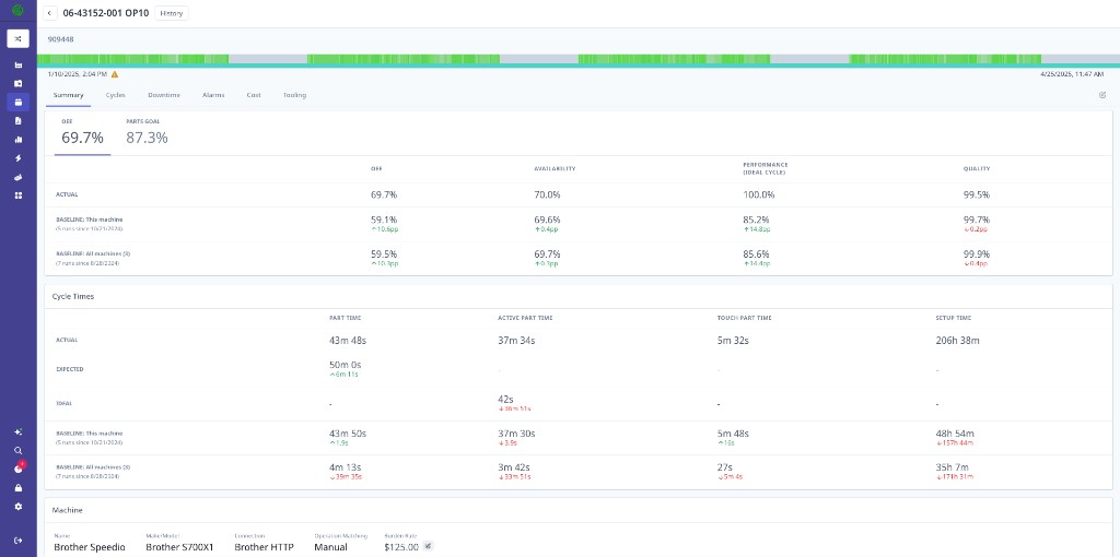
Summary Tab - Performance at a Glance
Overview
The Summary Tab provides a comprehensive overview of production performance for the selected operation, time period, and filters.
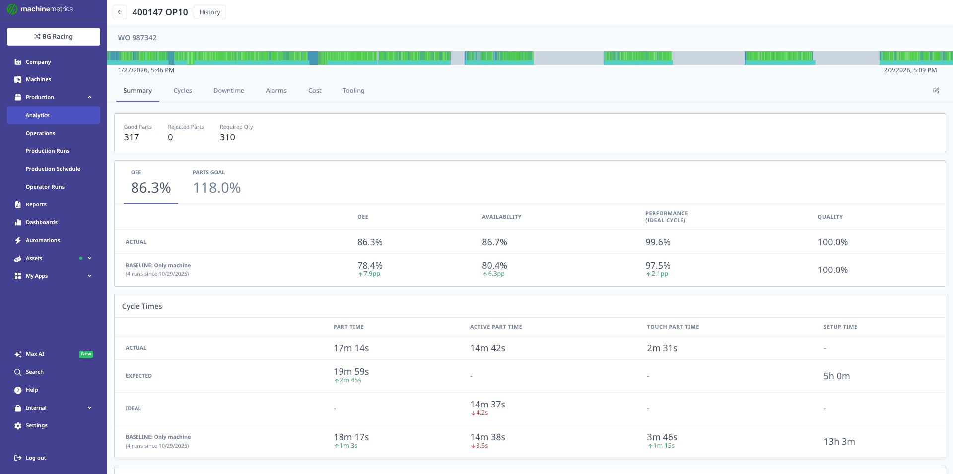
The Production Analytics Summary displays key metrics including parts produced (317 good, 0 rejected, 310 required), OEE breakdown (86.3% actual vs 118.0% parts goal), availability (86.7%), performance/ideal cycle (99.6%), quality (100.0%), and detailed cycle time analysis comparing actual, baseline, and expected performance.
Key Metrics Explained
Parts Produced:
- Good Parts: Successfully produced parts meeting quality standards
- Rejected Parts: Parts that failed quality checks
- Required Parts: Target quantity from work order (if specified)
- Parts Goal %: Progress toward required quantity
OEE (Overall Equipment Effectiveness):
- OEE %: Combined measure of Availability × Performance × Quality
- Availability %: (Time In Cycle / Scheduled Time) × 100
- Performance %: (Actual Parts × Ideal Cycle Time / Time In Cycle) × 100
- Quality %: (Good Parts / Total Parts) × 100
Cycle Time Analysis:
- Part Time: Total button-to-button time per part (actual)
- Active Part Time: Time machine was in-cycle per part
- Touch Part Time: Idle time per part — how much time the machine was stopped during each part cycle
- Setup Time: Total setup time for the run
Performance Comparisons:
- Actual vs Expected: How actual performance compares to ERP standard
- Actual vs Baseline: How current performance compares to historical baseline (plant average)
Business Insights from Summary
Quote Accuracy Check:
Expected Part Time: 15m 00s (ERP standard)
Actual Part Time: 17m 14s (median)
Variance: +14.9% slower than quoted

Impact: If you quoted 100 parts at 15 min/part = 25 hours
Reality: 100 parts at 17.25 min/part = 28.75 hours
Lost Time: 3.75 hours (15% underestimate)
Profitability Indicator:
OEE: 86.3%
This means 13.7% of scheduled time was lost to:
- Downtime (availability losses)
- Slow cycles (performance losses)
- Quality issues (quality losses)

If burden rate = $100/hour, scheduled time = 40 hours:
Cost of losses = $100 × 40 × 13.7% = $548
Capacity Planning:
Parts Required: 310
Parts Produced: 317
Parts Goal: 118.0% (exceeded target)

Availability: 86.7% (room for improvement)
Performance: 99.6% (excellent)
Quality: 100.0% (perfect)

Action: Focus improvement efforts on availability (downtime reduction)
to increase capacity without adding shifts.
Cycles Tab - Actual vs Planned Cycle Times
Overview
The Cycles Tab provides detailed cycle time analysis, showing the distribution of cycle times, statistical measures, and how actual times compare to expected standards.
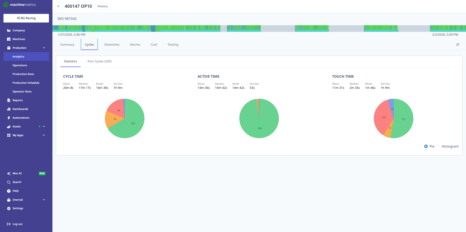
The Cycles tab displays three pie charts showing the distribution of cycle time, active time, and touch time across all part cycles. Statistical analysis includes median, mode, and 3rd standard deviation values. This example shows 329 cycles with consistent active times around 14m 42s, indicating a stable process.
Key Metrics
Statistical Measures:
- Median: Middle value (50th percentile) - most representative of typical cycle
- Mode: Most common cycle time - what the process runs at most often
- Mean: Mathematical average - useful for total time calculations
- Standard Deviation: Measure of variability - low = consistent, high = unstable
Cycle Time Types:
- Cycle Time: Total button-to-button time (load → unload → ready for next)
- Active Time: Time machine was actively cutting/processing
- Touch Time: Idle time within a cycle — time the machine was stopped while the operator was loading, unloading, or performing manual operations
Part Distribution:
- On-Target (Green): Cycles within acceptable range of expected time
- Slow (Yellow): Cycles moderately slower than expected
- Very Slow (Red): Cycles significantly slower than expected (investigate)
Business Insights from Cycles
Quote Validation:
ERP Standard: 15m 00s per part
Actual Median: 17m 14s per part
Actual Mode: 17m 10s per part
Variance: +14.9% slower than quoted

Analysis: The process consistently runs 2+ minutes slower than quoted.
This is NOT variability - the process is stable but the standard is wrong.

Action: Update ERP standard to 17m 15s/part for future quotes.
Process Stability Assessment:
Median: 17m 14s
Standard Deviation: 45 seconds

Range (±1 std dev): 16m 29s - 17m 59s
Coefficient of Variation: 4.4%

Analysis: Very stable process (CV < 5%). Low variability means:
- Predictable throughput for scheduling
- Reliable cycle time for quoting
- Process is in control

Action: Can confidently quote this operation with tight tolerances.
Outlier Investigation:
Mode: 17m 10s (most common)
Very Slow Parts (Red): 15 parts took 22m+ (30% slower)

Analysis: 95% of parts are consistent, but 5% have issues.

Potential Causes:
- Tool wear toward end of tool life
- Specific operator struggles
- Material hardness variation
- Machine warm-up cycles

Action: Filter by operator and time of day to identify root cause.
Capacity Impact:
Expected: 15 min/part × 500 parts = 125 hours
Actual: 17.25 min/part × 500 parts = 143.75 hours
Difference: 18.75 hours (15% more capacity required)

Impact:
- Need 18.75 more machine hours per job
- Affects scheduling and delivery promises
- Reduces available capacity for other work

Action: Either improve cycle time or adjust capacity planning.
Downtime Tab - Where Time Was Lost
Overview
The Downtime Tab identifies where production time was lost, categorizes reasons, and quantifies the impact. This is critical for understanding why actual time differs from planned time and where to focus improvement efforts.
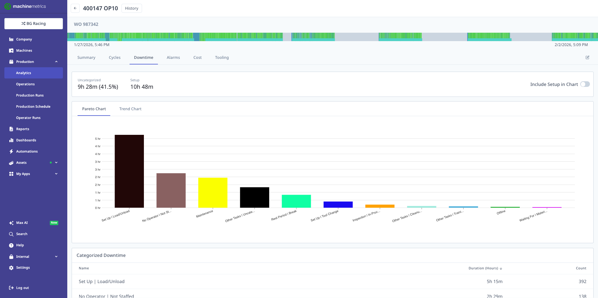
The Downtime tab shows a Pareto chart displaying top downtime reasons by duration. Total downtime is 9h 28m out of 10h 48m total time. In this example, "Set Up / Load/Unload" accounts for 5h 15m and "No Operator / Not Staffed" accounts for 7h 29m (note: time categories can overlap). Use this to identify the biggest opportunities for time savings.
Key Data
Downtime Categories:
- Setup / Changeover: Time setting up fixtures, tools, first article
- Waiting for Material: No material available to run
- Waiting for Operator: Machine idle, no operator present
- Tool Change / Tool Issues: Changing tools, broken tools, tool problems
- Maintenance / Repair: Unplanned breakdowns and repairs
- Quality Issues: Rework, inspection delays, scrap
- Other: Miscellaneous reasons
- Uncategorized: Downtime events without assigned reason
Visualizations:
- Pareto Chart: Top downtime reasons by total duration (80/20 rule)
- Downtime Table: All reasons with duration, count, and percentage
- Trend Chart: Downtime over time (improving or worsening?)
Business Insights from Downtime
Cost of Downtime:
Total Downtime: 9h 28m
Scheduled Time: 40 hours
Downtime %: 23.7%

If Burden Rate = $100/hour:
Cost of Downtime = $100 × 9.47 hours = $947

This cost was NOT in the original quote.
If quoted at 40 hours, actual cost is 23.7% higher.
Top Loss Identification (Pareto Principle):
Downtime by Category:
1. No Operator / Not Staffed: 7h 29m (79%)
2. Setup / Load/Unload: 5h 15m (55%)
3. Tool Issues: 1h 15m (13%)
4. All Others: 0h 30m (5%)

Note: Categories can overlap (machine idle = both "no operator" + "setup")

Analysis:
- 79% of downtime is "No Operator" - staffing issue
- 55% is setup/load/unload - could be reduced with fixtures or automation
- Focusing on top 2 reasons addresses 90%+ of downtime

Action Priority:
1. Improve staffing/scheduling (biggest impact)
2. Reduce setup time with fixtures
3. Then address tool issues
Quote Adjustment:
Planned Cycle Time: 15 min/part (in-cycle)
Actual Cycle Time: 17 min/part (including typical downtime)

Historical Downtime Average: 2 min per part cycle

Updated Quote Should Include:
- Cycle Time: 15 min/part (machine time)
- Downtime Allowance: 2 min/part (typical downtime)
- Total: 17 min/part

For 500 parts:
- Machine time: 125 hours
- Expected downtime: 16.7 hours
- Total quoted: 141.7 hours (vs original 125 hours)
Process Improvement ROI:
Current Setup Time: 5h 15m per job (315 minutes)
Target (Industry Best Practice): 2h 00m per job (120 minutes)
Potential Savings: 3h 15m per job (195 minutes)

If Burden Rate = $100/hour:
Savings per job = $100 × 3.25 hours = $325

If you run this job 12 times per year:
Annual savings = $325 × 12 = $3,900

ROI Calculation for Quick-Change Fixtures:
- Fixture cost: $5,000
- Payback period: 5,000 / 3,900 = 1.3 years
Alarms Tab - Machine Issues Impact
Overview
The Alarms Tab displays machine alarms and faults that occurred during production, showing which issues are most frequent or cause the longest delays.
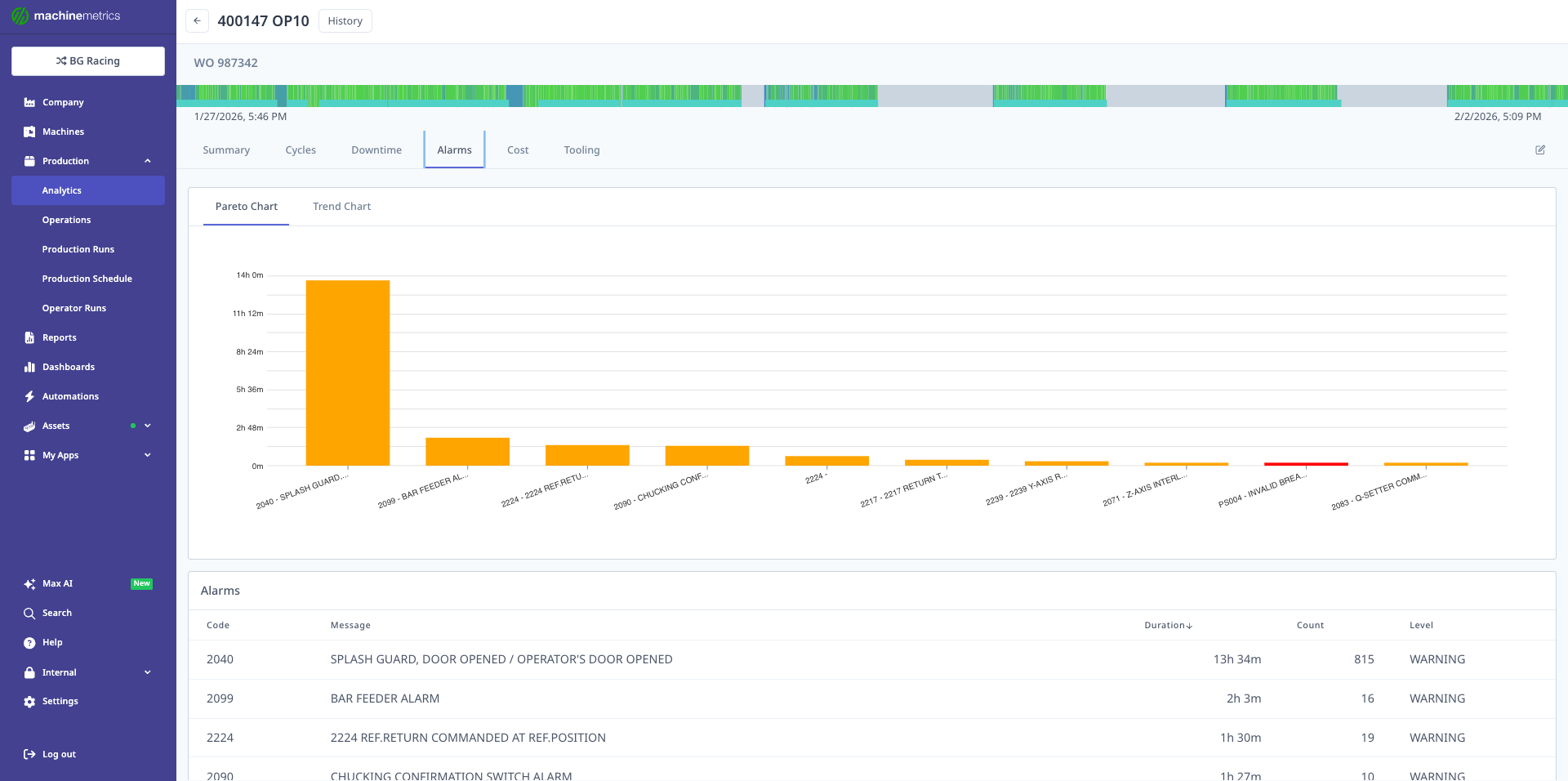
The Alarms tab shows a Pareto chart of top alarms by duration and a detailed table with alarm codes, messages, durations, counts, and severity levels. This example shows door/splash guard alarms (13h 34m total) and bar feeder alarms (2h 3m) as top issues. Use this to prioritize preventive maintenance and operator training.
Key Data
Alarm Information:
- Alarm Code: Machine-specific error or fault code
- Message: Description from machine control
- Duration: Total time alarm was active (downtime impact)
- Count: Number of times alarm occurred
- Severity: Warning, Fault, or Critical
- Time Pattern: When alarms occur (shift, operator, time of day)
Visualizations:
- Pareto Chart: Top alarms by duration or frequency
- Alarm Table: Detailed list of all alarms with metrics
- Trend Chart: Alarm patterns over time
Business Insights from Alarms
Recurring Issues:
Alarm: "Splash Guard/Door Opened"
Duration: 13h 34m (total across multiple occurrences)
Count: 127 times
Avg Duration: 6.4 minutes per occurrence

Analysis:
- Operator opening door mid-cycle (safety interlock)
- Possible causes: chip buildup, coolant issues, part inspection
- Very frequent but short duration

Impact on Quote:
- 127 door opens / 500 parts = 0.25 door opens per part
- 6.4 min avg × 0.25 = 1.6 min per part
- Adds 1.6 min × 500 parts = 800 minutes (13.3 hours) to job

Action:
- Operator training (reduce unnecessary door opens)
- Improve chip management (reduce need to open door)
- Could save 50% = 6.7 hours per job
Preventive Maintenance Opportunity:
Alarm: "Bar Feeder Fault"
Duration: 2h 3m
Count: 8 times
Avg Duration: 15.4 minutes per occurrence

Analysis:
- Bar feeder failing intermittently
- Likely mechanical wear or adjustment needed
- Each fault = 15+ minutes downtime

Annual Impact (if runs 12x/year):
- 2 hours × 12 = 24 hours downtime/year
- Cost = 24 hours × $100/hour = $2,400/year

Action:
- Schedule PM on bar feeder ($500 service)
- Payback in 3 months if eliminates faults
Operator Training Need:
Filter by Operator:

Operator A: 45 alarms, 3h 15m total
Operator B: 89 alarms, 7h 30m total ← Issue
Operator C: 38 alarms, 2h 45m total

Analysis:
- Operator B has 2× the alarm rate of others
- Possible causes: less experience, poor technique, rushing

Impact: Operator B costs an extra 5 hours/job in alarm downtime

Action: Training or mentoring to reduce alarm rate
Potential savings: 5 hours × 12 jobs × $100 = $6,000/year
Setting the Burden Rate
The Cost tab will show $0.00 for all financial metrics until a burden rate is entered. This is the most common reason cost data appears blank.
What Is the Burden Rate?
The burden rate is your fully-loaded machine cost per hour — the dollar amount it costs your shop to run a machine for one hour, including labor, overhead, depreciation, and utilities. MachineMetrics multiplies this rate by actual machine time to calculate the true cost of each production run.
Example: If your burden rate is $125/hour and a job takes 2 hours of actual machine time, the per-part cost (for a 100-part run) is:
$125 × 2h ÷ 100 parts = $2.50 per part
This figure populates the Cost tab metrics including Per Part Cost, Touch Time Cost, and the UEE loss breakdown.
Where to Find and Set the Burden Rate
The burden rate is set per operation inside the Operation Summary screen. There is no global setting — you must open each individual operation and enter the rate directly in the Cost tab.
Step 1: Open an operation
Navigate to Production Analytics and click into any operation (e.g., a specific part number and operation number).
The Operation Summary screen. The tabs across the top (Summary, Cycles, Downtime, Alarms, Cost, Tooling) are visible once you click into a specific operation.
Step 2: Click the Cost tab
Select the Cost tab at the top of the Operation Summary screen.
Step 3: Enter the burden rate at the bottom of the page
Scroll to the bottom of the Cost tab. You will see a Hourly Burden Rate field showing the machine name and current rate. Click the edit icon (pencil) next to the dollar amount and enter your burden rate.
The burden rate field is at the very bottom of the Cost tab, labeled "Hourly Burden Rate of [Machine Name]." In this example the rate is set to $125.00/hour. All cost figures on the page are calculated from this value.
The burden rate must be set individually for each operation. Updating one operation does not apply the rate to other operations, even for the same machine.
Step 4: Save and verify
After entering the rate, save the change. The Cost tab metrics — Per Part Cost, Touch Time Cost, UEE Losses, and Cycle Time Costs — will immediately recalculate using the new rate.
Required Permissions
You need Admin or Manager level access to edit the burden rate. Operator-level users can view the Cost tab but cannot modify the rate.
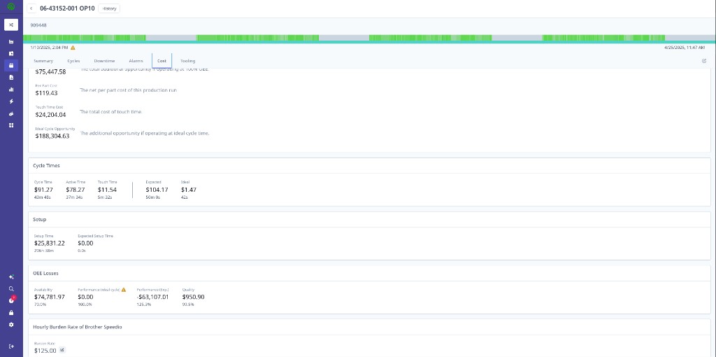
Cost Tab - True Profitability Analysis
Overview
The Cost Tab is the heart of Production Analytics for CFOs and estimators. It translates performance data into dollars, showing true per-part cost, cost of losses, and profitability.
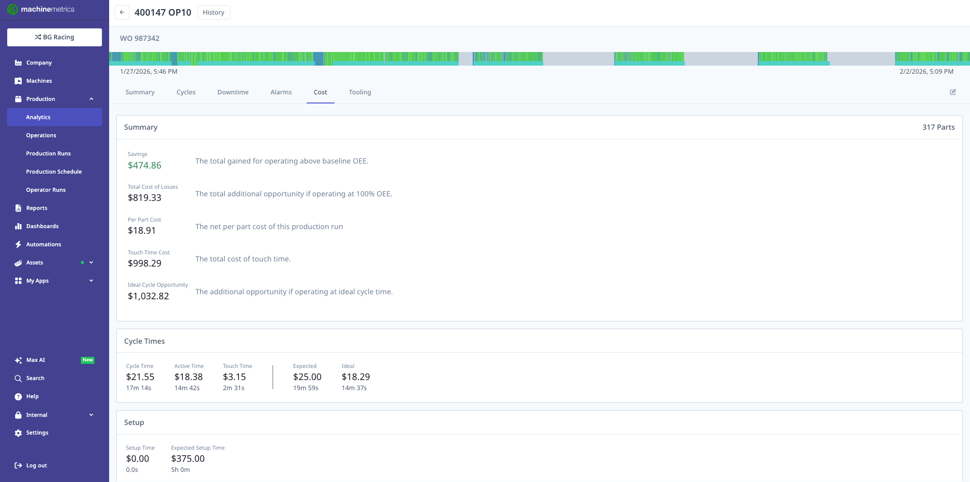
The Cost tab displays financial impact metrics: Gained ($474.86 - operating above baseline OEE), Ideal Cycle Losses ($819.33 - opportunity if at 100% OEE), Per Part Cost ($18.91 - net cost this run), Touch Time Cost ($998.29 - cost of operator touch time), and Idle Cycle Opportunity ($1,032.82 - opportunity if at ideal cycle time). The cycle times breakdown shows expected, actual, and baseline times with associated costs.
Key Metrics
Performance vs Baseline:
- Gained: Additional profit from operating above baseline OEE
- Lost: Cost of operating below baseline OEE
- Baseline: Historical average performance for comparison
Cost Components:
- Per Part Cost: Net cost per part produced (burden rate × actual time / parts)
- Touch Time Cost: Total cost of machine idle time within cycles
- Idle Cycle Opportunity: Potential savings if eliminating idle time in cycles
Loss Analysis:
- Ideal Cycle Losses: Cost of operating below 100% OEE
- Availability Losses: Cost of downtime
- Performance Losses: Cost of slow cycles
- Quality Losses: Cost of rejected parts
Cycle Time Costs:
- Expected Time: Cost if running at ERP standard
- Actual Time: True cost of actual performance
- Baseline Time: Cost at historical average
- Ideal Time: Cost if running perfectly (no losses)
Business Insights from Cost Tab
True Per-Part Cost:
Quote (Expected):
- Expected Part Time: 15 min/part
- Burden Rate: $100/hour
- Quoted Cost: $25.00/part

Actual:
- Actual Part Time: 17.25 min/part
- Burden Rate: $100/hour
- Actual Cost: $28.75/part

Variance: +$3.75/part (+15% cost overrun)

Job Impact (500 parts):
- Quoted Cost: $12,500
- Actual Cost: $14,375
- Loss: $1,875 (15% margin erosion)

Action: Update future quotes to $28.75+/part or improve process to meet $25/part target.
Cost of Losses Breakdown:
Total Losses: $1,875 (from 15% performance gap)

By Category:
- Availability Losses: $1,200 (64%) - downtime cost
- Performance Losses: $450 (24%) - slow cycles
- Quality Losses: $225 (12%) - scrap/rework

Analysis: Downtime is the biggest cost driver (64% of losses)

Improvement Priorities:
1. Reduce downtime (setup, operator availability)
2. Optimize cycle time (feeds/speeds, tooling)
3. Improve first-pass yield (quality)
Profitability Analysis:
Customer Price: $45.00/part
Quoted Cost: $25.00/part
Quoted Margin: $20.00/part (44.4% margin)

Actual Cost: $28.75/part
Actual Margin: $16.25/part (36.1% margin)

Margin Impact:
- Planned Profit: $20 × 500 = $10,000
- Actual Profit: $16.25 × 500 = $8,125
- Lost Profit: $1,875 (18.75% erosion)

Business Impact:
- If you run this job 12 times/year
- Annual lost profit: $1,875 × 12 = $22,500

Action: Either improve process or adjust pricing on next quote.
Opportunity Value:
Idle Cycle Opportunity: $1,032.82

This represents potential savings if you could eliminate:
- Operator wait time during cycle
- Load/unload delays
- In-cycle idle time

Potential Solutions:
- Automation (robot loading)
- Fixture improvements (faster load/unload)
- Operator multi-machine assignment

ROI Example:
- Robot cell cost: $75,000
- Annual savings (12 jobs): $1,033 × 12 = $12,396
- Additional capacity freed: 20% (can take more work)
- Payback: 6 years on savings alone, faster with new revenue
Baseline Comparison:
Gained: $474.86 (operating above plant baseline)

Analysis: This job performed better than typical jobs at this facility
- Baseline OEE: ~75% (typical)
- Actual OEE: 86.3% (this job)
- Performance gap: +11.3 percentage points

Why did this job perform better?
- Experienced operator
- Well-maintained machine
- Good tooling
- Adequate material supply

Action: Document what went right, replicate on other jobs.
Tooling Tab - Tool Performance
Overview
The Tooling Tab provides detailed analysis of tool usage, helping identify tool wear, inefficiencies, and opportunities for tool life optimization.
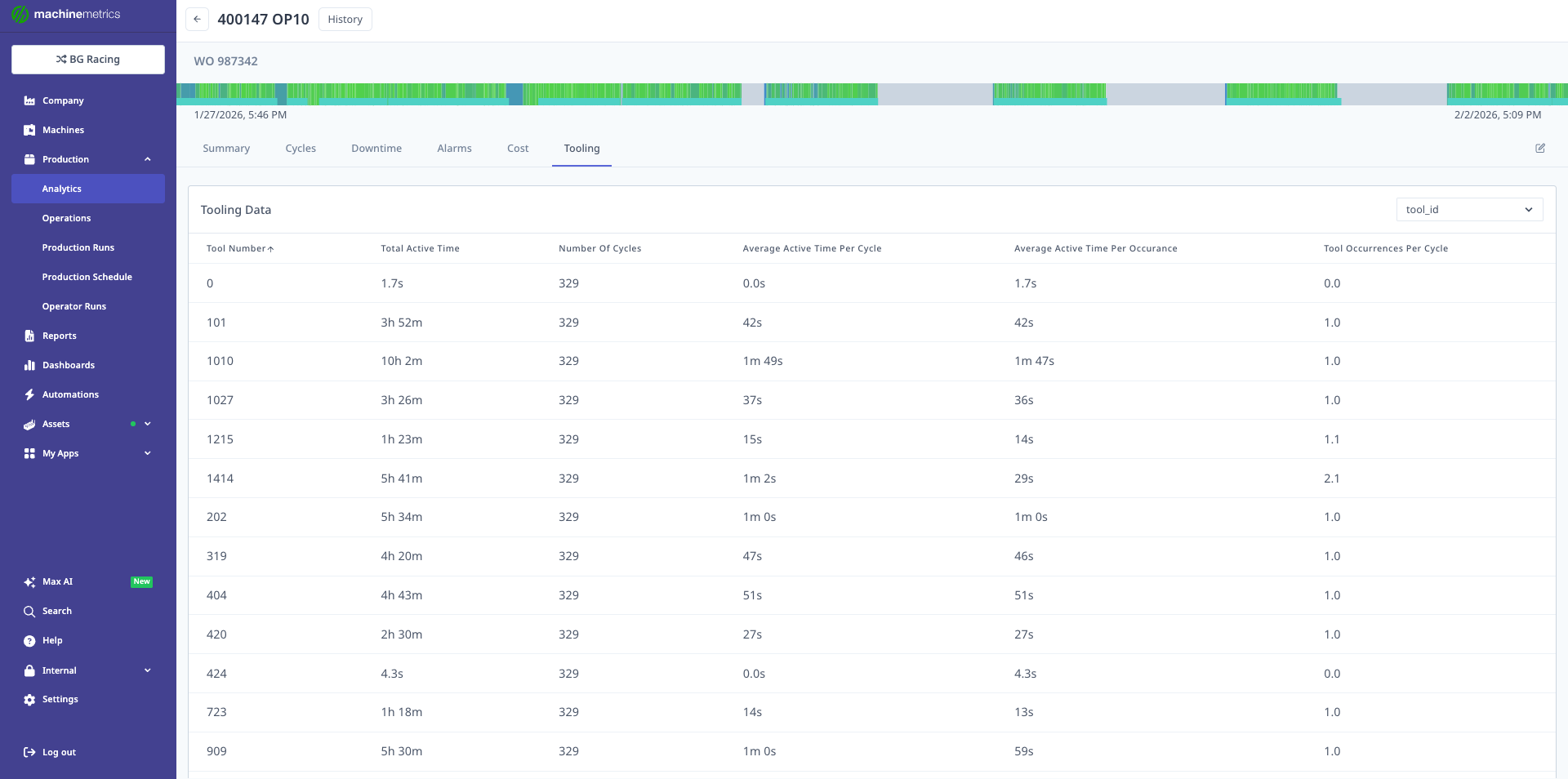
The Tooling tab displays comprehensive tool usage data across 329 cycles, showing tool number, total active time, number of cycles, average active time per cycle, average active time per occurrence, and tool occurrences per cycle. Use this to identify tool performance patterns, detect wear indicators, and optimize tool life.
Key Metrics
Tool Usage Data:
- Tool Number: Machine tool position or identifier
- Total Active Time: Cumulative time tool was in use
- Number of Cycles: How many cycles used this tool
- Avg Active Time per Cycle: Average time tool is used per part
- Tool Occurrences per Cycle: How many times tool is called per part
Performance Indicators:
- Increasing Cycle Time: Tool wear causing slower cuts
- Decreasing Frequency: Tool being skipped (possible tool failure)
- Variability: Inconsistent tool usage (process instability)
Business Insights from Tooling
Tool Wear Detection:
Tool #5 - Finish Boring Tool

Cycles 1-100: Avg 2m 15s per cycle
Cycles 101-200: Avg 2m 18s per cycle (+2.2%)
Cycles 201-300: Avg 2m 24s per cycle (+6.7%)
Cycles 301-329: Avg 2m 32s per cycle (+12.6%)

Analysis: Clear tool wear pattern, cycle time increasing over tool life

Impact on Quote:
- Fresh tool: 2m 15s per part
- Worn tool: 2m 32s per part
- Average: 2m 23s per part (should use for quotes)

If quoting with fresh tool time:
- 500 parts × 7 seconds lost per part = 58 minutes underestimated
Tool Life Optimization:
Tool #8 - Drill

Manufacturer Recommendation: 5,000 cycles
Current Practice: 3,500 cycles (conservative replacement)

Cost Analysis:
- Tool cost: $125
- Cost per cycle (current): $125 / 3,500 = $0.036/part
- Cost per cycle (at 5,000): $125 / 5,000 = $0.025/part
- Potential savings: $0.011/part

If running 50,000 parts/year:
- Current tool cost: $0.036 × 50,000 = $1,800/year
- Optimized tool cost: $0.025 × 50,000 = $1,250/year
- Savings: $550/year per tool

Action: Monitor tool performance, push tool life closer to recommended limit.
Tool Change Frequency:
Tool #12 - Face Mill Insert

Occurrences per Cycle: 4.2
Expected per Part: 2.0
Variance: 210% (tool used 2× more often than expected)

Possible Causes:
- Tool re-touching mid-cycle (wear issue)
- Program inefficiency (multiple tool calls)
- Incorrect CAM programming

Impact:
- Extra tool usage = premature wear
- Longer cycle time (tool changes add time)

Action: Review program, optimize tool path, investigate wear.
Optimizing Your Quoting Process
Workflow for Quote Improvement
Step 1: Run the Job
- Produce the part with current standards
- Let MachineMetrics capture all data automatically
- Complete the production run
Step 2: Analyze Performance
- Navigate to Production → Analytics
- Filter to the specific operation
- Review all tabs:
- Summary: Overall performance vs expected
- Cycles: Actual cycle time distribution
- Downtime: Where time was lost
- Cost: True per-part cost
Step 3: Compare to History
- Click History button
- Compare current run to previous runs
- Identify trends:
- Are we getting faster or slower?
- Is OEE improving or declining?
- Are downtime patterns consistent?
Step 4: Calculate True Costs
- Use Cost Tab data to determine:
- True per-part cost (including losses)
- Cost of typical downtime
- Impact of performance variance
- Add realistic profit margin
- Calculate customer price
Step 5: Update ERP Standards
- Update cycle time to actual median (from Cycles Tab)
- Update setup time to actual average (from Downtime Tab)
- Add downtime allowance based on historical average
- Document in ERP system for future quotes
Step 6: Identify Improvement Opportunities
- From Downtime Tab: Top 3 downtime reasons
- From Alarms Tab: Most frequent or costly alarms
- From Cycles Tab: Process stability (high variability?)
- Calculate ROI for potential improvements
Step 7: Monitor and Iterate
- Run job again with improvements
- Use History to validate improvement impact
- Update quotes if performance improves
- Continue cycle of analysis and improvement
Real-World Example
Initial Quote (Before Production Analytics):
Part: Housing Assembly (Part #1077280)
Operation: Rough Turn (OP10)

Quoted Parameters:
- Cycle Time: 15 min/part (ERP standard, last updated 3 years ago)
- Setup Time: 30 min
- Quantity: 500 parts
- Total Time: 30 min + (15 min × 500) = 125.5 hours
- Burden Rate: $100/hour
- Quoted Cost: $12,550
- Price to Customer: $20,000 (59% margin)
After First Production Run (Production Analytics Data):
Actual Performance:
- Actual Cycle Time: 17.25 min/part (median)
- Actual Setup Time: 65 min
- Actual Downtime: 9.5 hours (tool changes, waiting for operator)
- Total Time: 65 min + (17.25 min × 500) + 9.5 hours = 153.8 hours

True Cost: $15,380
Actual Margin: $20,000 - $15,380 = $4,620 (23% margin, not 59%)
Lost Profit: $7,930 (63% margin erosion)
Root Cause Analysis:
From Production Analytics:

1. Cycle Time Variance (+2.25 min/part):
   - Tool wear slowing cycles
   - Operator less experienced than expected
   - Result: +18.75 hours

2. Setup Time Variance (+35 min):
   - Fixture took longer to locate/align
   - First article inspection extended
   - Result: +0.58 hours

3. Unplanned Downtime (+9.5 hours):
   - Tool changes: 4.5 hours (16 tool changes)
   - Waiting for operator: 3.0 hours (lunch, breaks not covered)
   - Material delays: 2.0 hours (bar stock ran out)
   - Result: +9.5 hours

Total Variance: 28.3 hours (22.5% over quote)
Improvement Actions:
1. Immediate (For Next Quote):
   - Update ERP standard to 17.25 min/part
   - Update setup time to 65 minutes
   - Add 10% contingency for downtime
   - New quote: 153.8 × 1.0 = 153.8 hours
   - New cost: $15,380
   - New price: $22,000 (43% margin)

2. Short-Term (Process Improvements):
   - Purchase better tooling (reduce tool changes by 50%)
   - Improve fixture (reduce setup time to 40 min)
   - Train operator (reduce cycle time to 16 min/part)

   Expected Results:
   - Cycle time: 16 min/part
   - Setup: 40 min
   - Tool changes: 2.25 hours (50% reduction)
   - Total: 135.9 hours
   - Cost: $13,590
   - Margin improvement: $1,790 vs current

3. Long-Term (Competitive Advantage):
   - Quote accurately, win more bids
   - Improve processes, increase margins
   - Use data to justify pricing to customers
After Improvements (6 Months Later):
Production Analytics Shows:
- Cycle Time: 16m 10s (6.5% improvement)
- Setup Time: 42 min (35% improvement)
- Tool Change Downtime: 2.5 hours (72% improvement)
- Total Time: 138.2 hours (10% improvement)

Financial Impact:
- Cost: $13,820
- Margin: $22,000 - $13,820 = $8,180 (37% margin)
- Improvement: +$3,560 profit per job vs initial actual

If running 12 times/year:
- Annual profit improvement: $42,720
- Plus: Freed capacity = 187 machine hours/year (more revenue potential)
Filtering and Exporting Data
Filtering Options
Available Filters:
- Date Range:
- Presets: Today, Yesterday, Last 7 Days, Last 30 Days, This Month, Last Month
- Custom: Select any start and end date
- Machines: Filter to specific machines or machine groups
- Operations: Filter to specific part/operation combinations
- Shifts: Filter to specific shifts (1st, 2nd, 3rd, weekend)
- Operators: Filter to specific operators (requires Operator Insight feature)
- Activities: Include or exclude setup time vs production time
Using Filters:
- Click filter controls at top of Production Analytics page
- Select desired filter values
- Click Apply or Update button
- All tabs update with filtered data
- Filters remain active when switching between tabs
Common Filter Use Cases:
Use Case: Compare shift performance
- Date Range: Last 30 Days
- Machines: All CNC Lathes
- Shift: First Shift vs Second Shift
- Compare: OEE, cycle times, downtime reasons

Use Case: Operator training effectiveness
- Operation: Specific part operation
- Date Range: Last 90 Days
- Operator: Compare trainee vs experienced operators
- Analyze: Cycle time improvement over time

Use Case: Machine capability study
- Date Range: Last 7 Days
- Operation: Specific operation
- Machines: Compare multiple machines running same part
- Analyze: Which machine has best OEE and cycle time consistency

Use Case: Historical trend analysis
- Operation: Long-running production part
- Date Range: Last 12 Months
- View: Month-over-month performance trends
- Identify: Seasonal patterns, degradation, improvements
Exporting Data
Export Formats:
- CSV: Raw data for Excel analysis, pivot tables, custom reports
- PDF: Formatted report for printing or email distribution
Export Steps:
- Configure filters to show desired data
- Navigate to tab you want to export (Summary, Cycles, Downtime, etc.)
- Click Export button (usually top-right)
- Select format (CSV or PDF)
- File downloads to your computer
CSV Export Use Cases:
1. Executive Reports:
   - Export Summary tab to CSV
   - Import into Excel
   - Create custom dashboard for CFO
   - Include: OEE trends, cost analysis, profitability

2. Deep Dive Analysis:
   - Export Cycles tab raw data
   - Statistical analysis in Excel or Minitab
   - Six Sigma analysis (Cp, Cpk calculations)
   - Process capability studies

3. Benchmarking:
   - Export same operation across multiple machines
   - Compare performance in Excel pivot tables
   - Identify best performers
   - Share best practices

4. ERP Updates:
   - Export actual cycle times
   - Update ERP standards database
   - Import new standards into planning system
PDF Export Use Cases:
1. Quote Documentation:
   - Export Production Analytics for specific job
   - Attach to quote as justification
   - Show customer historical performance data
   - Demonstrate capability and consistency

2. Customer Reporting:
   - Export performance summary for contract manufacturer
   - Send monthly performance reports
   - Document OEE and quality metrics
   - Transparency builds trust

3. Management Reviews:
   - Print PDF reports for monthly operations meetings
   - Review year-over-year improvements
   - Discuss investment priorities
   - Track KPI progress
Scheduled Reports:
Some organizations set up automated scheduled reports:
- Daily OEE summary emailed to managers
- Weekly downtime Pareto to maintenance team
- Monthly cost analysis to CFO
- Quarterly performance review to executive team
Note: Scheduled reporting is configured in System Settings → Reports. Contact your MachineMetrics administrator to set up automated reports.
Getting Help
Common Questions
"My OEE seems wrong"
Possible Causes:
- Scheduled time not configured correctly (are shifts assigned to machines?)
- Expected part time in operation is inaccurate
- Planned downtime not marked correctly
How to Troubleshoot:
- Check Summary Tab → Review OEE components (A/P/Q)
- Which component is unexpected?
- Availability low? Check downtime and scheduled time
- Performance low? Check expected vs actual cycle time
- Quality low? Check rejected parts count
- Verify operation settings in Production → Operations
"Cycle times don't match reality"
Possible Causes:
- Part counting method incorrect (1 per cycle vs multiple per cycle)
- Touch time included when you expected only active time
- Setup time mixed with production time
How to Troubleshoot:
- Review Cycles Tab → Check cycle time vs active time vs touch time
- Filter Activities to exclude setup if analyzing only production
- Verify part counting configuration in operation settings
"Cost data doesn't appear" / all cost values show $0.00
Most Likely Cause: No burden rate has been entered for this operation.
How to Fix:
- Open the operation in Production Analytics
- Click the Cost tab at the top of the Operation Summary screen
- Scroll to the bottom of the Cost tab
- Find the Hourly Burden Rate field (labeled with the machine name)
- Click the edit icon and enter the rate (e.g., $125.00/hour)
- Save — all cost metrics will recalculate immediately
Note: The burden rate is set per operation, not globally. Each operation needs its own rate entry. See the Setting the Burden Rate section above for full details.
"Historical data is missing"
Possible Causes:
- Operation was archived or deleted
- Production runs were not tracked during that period
- Date range filter excluding desired period
How to Troubleshoot:
- Check date range filter (expand to wider range)
- Verify production runs exist: Production → Production Runs
- Check if operation was archived: Production → Operations → Show Archived
- If data truly missing, may need manual entry or accept gap
"Can't compare operators"
Possible Causes:
- Operator Insight feature not enabled
- Operators not logging in on tablets
- Operator runs not assigned
How to Troubleshoot:
- Verify Operator Insight is enabled: Settings → Company Settings
- Check operator login: Review operator dashboard usage
- Assign operators retroactively: Production → Operator Runs
Best Practices for Quote Optimization
1. Start with Stable Operations
- Begin analyzing operations you run frequently (weekly or monthly)
- High-volume parts provide more data for reliable trends
- Low-mix, high-volume operations are easiest to benchmark
2. Build Historical Baseline
- Run operation at least 3-5 times before updating quotes
- Use median values, not single runs (eliminates outliers)
- Account for operator learning curve (early runs may be slower)
3. Include Realistic Contingency
- Add 5-10% contingency for variability
- Manufacturing is never perfect
- Contingency protects margin on difficult runs
4. Review Quarterly
- Set calendar reminder to review Production Analytics quarterly
- Update ERP standards based on latest data
- Track improvement progress over time
5. Document Assumptions
- Record why you quoted specific times
- Note any process changes between runs
- Create audit trail for future reference
6. Collaborate Across Teams
- Estimators: Use data to improve quote accuracy
- Process Engineers: Identify improvement opportunities
- Finance: Understand true costs and margins
- Operations: Validate data accuracy
Contact Support
MachineMetrics Support:
- Email: support@machinemetrics.com
- Include:
- Operation name(s)
- Machine name(s)
- Date range you're analyzing
- Screenshot of the specific issue
- What you expected vs what you're seeing
For Training:
- Request Production Analytics training session
- Ask about advanced filtering and analysis techniques
- Schedule CFO/estimator-focused workshop
- Request quote optimization consulting
Ready to optimize your quoting?
- Navigate to Production → Analytics
- Select an operation you run frequently
- Click History to see past performance
- Compare actual vs expected in Summary and Cost tabs
- Use real data to update your next quote
Questions? Contact support@machinemetrics.com